Foundations of Machine Learning I
Lately, I was into the studying process of machine learning, and outputting(taking notes) is a vital step of it. Here, I am using Andrew Ng’s Stanford Machine Learning course in Coursera with the language of MATLAB.
So the rest of the code I will write in this post by default are based on MATLAB.
What is ML?⌗
“A computer program is said to learn from experience E with respect to some class of tasks T and performance measure P, if its performance at tasks in T, as measured by P, improves with experience E.” Tom Mitchell
Supervised Learning&Unsupervised Learning
SL: with labels; direct feedback; predict
Under SL, there are regression and classification
USL: without labels; no feedback; finding the hidden structure
Under USL, there are clustering and non-clustering
For now, I would focus on these two but not reinforcement learning.
The Basic Model & Notation⌗
We use $x^{(i)}$ to represent the “input” value, with the variable $x$ represent the value at the position $i$ in a matrix , or vector in most of the time. And $y^{(i)}$ is the actual “output” when we have a input $x$ at position variable $i$. A pair of $(x^{(i)}, y^{(i)})$ is called a training sample. Then we have a list of such samples with $i=1,…,m$—is called a training set. And the purpose of ML is to have a “good” hypothesis function $h(x)$ which could predict the output while only knowing the input $x$. If we only want to have a simple linear form of $h(x)$, then it looks like: $h(x)=\theta_0 + \theta_1x$, which both $\theta_0$ and $\theta_1$ is the parameter we want to find that letting $h(x)$ to predict “better”.
Linear Algebra Review⌗
Matrix-Vector Multiplication:$\begin{bmatrix} a & b \newline c & d \newline e & f \end{bmatrix} * \begin{bmatrix} x \newline y \end{bmatrix} = \begin{bmatrix} a*x + b*y \newline c*x + d*y \newline e*x + f*y \end{bmatrix}$
Matrix-Matrix Multiplication: $\begin{bmatrix} a & b \newline c & d \newline e & f \end{bmatrix} * \begin{bmatrix} w & x \newline y & z \newline \end{bmatrix}=\begin{bmatrix} a*w + b*y & a*x + b*z \newline c*w + d*y & c*x + d*z \newline e *w + f*y & e*x + f*z \end{bmatrix}$
Identity Matrix looks like this—with 1 on the diagonal and the rest of the elements are zeros: $\begin{bmatrix} 1 & 0 & 0 \newline 0 & 1 & 0 \newline 0 & 0 & 1 \newline \end{bmatrix}$
eye(3)
Multiplication Properties
Matrices are not commutative: $A∗B \neq B∗A$
Matrices are associative: $(A∗B)∗C = A∗(B∗C)$
Inverse and Transpose
Inverse: A matrix A mutiply with its inverse A_inv results to be a identity matrix I:
I = A*inv(A)
Transposition is like rotating the matrix 90 degrees, for a matrix A with dimension $m * n$, its transpose is with dimension $n * m$:
$$A = \begin{bmatrix} a & b \newline c & d \newline e & f \end{bmatrix}, A^T = \begin{bmatrix} a & c & e \newline b & d & f \newline \end{bmatrix}$$
Also we can get:
$$A_{ij}=A_{ji}^{T}$$
Cost Function⌗
A cost function shows how accurate our hypothesis function predict while output the error (the deviation between $y(x)$ and $h(x)$). And it looks like this:
$$ J(\theta_0, \theta_1) = \dfrac {1}{2m} \displaystyle \sum_{i=1}^m \left (h_\theta (x^{(i)}) - y^{(i)} \right)^2 $$
For people who are familier with statistics, it is called “Squared error funtion” while the square makes each error becomes a positice value, and the $\frac{1}{2}$ helps to simplify the expression later when we do derivative during the process of gradient descent. Now, we turn the question to “How to find $\theta_0, \theta_1$ that minilize $J(\theta_0, \theta_1)$?”
Contour Plot⌗
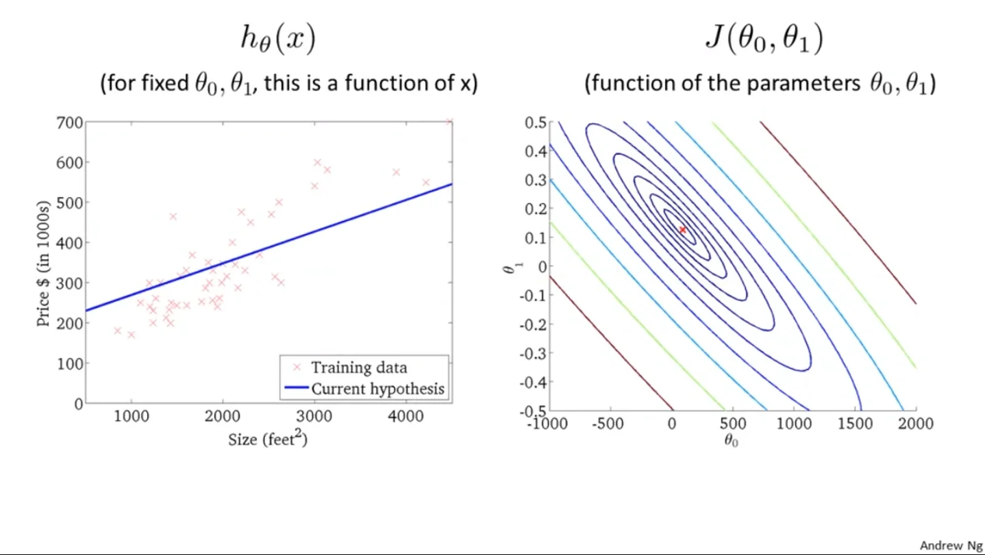
$J(\theta_0, \theta_1)$ in contour plot From Andrew Ng
A contour plot is actually an alternative way to show 3D graphs in 2D, in which the color blue represents low points while red means the high. So the $J(\theta_0, \theta_1)$ that gives the red point is the set of the parameter gives $h(x)$ with the lowest error with the actual output $y(x)$
Gradient Descent⌗
Gradient Descent is one of the most basic ML tools. The basic idea is to “move some small steps which lead to minimizing the cost function $J(\theta)$. And it looks like this:
Repeat until convergence:
{
$\theta_j := \theta_j - \alpha \frac{\partial}{\partial \theta_j} J(\theta_0, \theta_1)$
}
Here, the operator $:=$ just means assign the latter part to the former part while we know it could be the same as $=$ in many languages. We say the former $\theta_j$ as the “next step” while the latter one as the “current position”, $\frac{\partial}{\partial \theta_j} J(\theta_0, \theta_1)$ shows the “direction” that make the move increase $J(\theta)$ the most, so that we could just add a negative sign to make it becomes the fastest decrease direction.$\alpha$ gives the length of step we want it to take for each step. And it’s important to make the update of each $\theta$ be simultaneous.
If we take the code above apart, then we have:
repeat until convergence:
{
$\theta_0 := \theta_0 - \alpha \frac{1}{m} \sum\limits_{i=1}^{m}(h_\theta(x^{(i)}) - y^{(i)})$
$\theta_1 := \theta_1 - \alpha \frac{1}{m} \sum\limits_{i=1}^{m}((h_\theta(x^{(i)}) - y^{(i)}) x^{(i)})$
}
The term $x_i$ is nothing but a result of the derivative, there is no $x_i$ for $\theta_0$ because we defined $x^{(i)}_0$ as 1.
Then here is a full derivative process to show the partial dervative of the cost function $J(\theta)$:
$$\begin{aligned}\frac{\partial }{\partial \theta_j}J(\theta) &= \frac{\partial }{\partial \theta_j}\frac{1}{2}(h_\theta(x)-y)^{2}\newline&=2 \cdot \frac{1}{2}(h_\theta(x)-y) \cdot \frac{\partial }{\partial \theta_j}(h_\theta(x)-y)\newline&= (h_\theta(x)-y)\frac{\partial }{\partial \theta_j}\left ( \sum\limits_{i=0}^n\theta^{(i)}x^{(i)}-y \right )\newline&=(h_\theta(x)-y)x_j\end{aligned}$$
And such basic method is called batch gradient descent while it uses all the training set we provide, and just saying for future reference, $J(\theta)$is convex which means it only has only one global minima and has no chance to be affected by local minima.
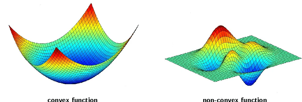
Convex function&non-convex function
Multivariate Linear Regression⌗
So saying we have not only one variables of input, but many of them. Then we use $j$ in $x_j$ from 1 to $n$ to represents the index of it just like we use $i$ to represents the index of the training example from 1 to $m$.
$x_{j}^{(i)}$ = value of, in $i^{th}$ training example, feature $j$
For convenience of notation, we have to define $x_0 = 1$, since we have $\theta_0$ in the hypothesis function, and the matrix mutiplication thing:
$$x = \begin{bmatrix} x_1 \newline x_2 \newline \vdots \newline x_n \end{bmatrix} \in \mathbb{R}^{n} , \theta = \begin{bmatrix}\theta_0 \newline \theta_1 \newline \theta_2 \newline \vdots \newline \theta_n \end{bmatrix} \in \mathbb{R}^{n+1} \rightarrow x = \begin{bmatrix}x_0 \newline x_1 \newline x_2\newline \vdots \newline x_n \end{bmatrix} \in \mathbb{R}^{n+1}, \theta = \begin{bmatrix}\theta_0 \newline \theta_1 \newline \theta_2\newline \vdots \newline \theta_n \end{bmatrix} \in \mathbb{R}^{n+1}$$
And the cool thing here we can do now is using vectorization to represents the long mutivariable hypothesis function:
$$h_\theta (x) = \theta_0 + \theta_1 x_1 + \theta_2 x_2 + \theta_3 x_3 + … + \theta_n x_n = \begin{bmatrix}\theta_0&\theta_1&\cdots&\theta_n\end{bmatrix}\begin{bmatrix}x_0 \newline x_1 \newline \vdots \newline x_n\end{bmatrix}=\theta^T x$$
Feature Scaling
If the input set $x$ contains features that have very large difference on their data range, the process of getting $\theta$ could oscillating, being slow, or even failed, and feature scaling, or mean normalization is a technique to make the range of data in each feature more even, and the process is very familir if knowing statistics:
$$x_j:=\frac{x_j-\mu_j}{s_j}$$
So the input $x$ with feature index $j$ minus the mean of the data in this feature then divided by the standard deviation(or range in some cases)
Normal Equation
Other than gradient descent, there is another way to find the minimized cost function$J(\theta)$. We first need to construct a matrix $X$ which is a another way to show the input data set of $x$:
$$x = \begin{bmatrix}x_0 \newline x_1 \newline x_2 \newline \vdots \newline x_n \end{bmatrix} \rightarrow X = \begin{bmatrix} x^{(1)}_0 & x^{(1)}_1 & \cdots & x^{(1)}_n \newline x^{(2)}_0 & x^{(2)}_1 & \cdots & x^{(2)}_n \newline \vdots & \vdots & \ddots & \vdots \newline x^{(m)}_0 & x^{(m)}_1 & \cdots & x^{(m)}_n \end{bmatrix} =\begin{bmatrix} 1 & x^{(1)}_1 & \cdots & x^{(1)}_n \newline 1 & x^{(2)}_1 & \cdots & x^{(2)}_n \newline \vdots & \vdots & \ddots & \vdots \newline 1 & x^{(m)}_1 &\cdots & x^{(m)}_n \end{bmatrix} $$
Actually, each row of the matrix $X$ is the transpose of each element in $x_j^{(i)}$, contains the data set for all features in one iteration. And the normal equation itself looks like:
$$\theta = (X^{T}X)^{-1}X^{T}y$$
I am not going to show how it comes but comparing to gradient descent, the normal equation: 1. no need to choose $\alpha$ 2. no need to iterate 3. but slow.
Classification⌗
Not only we need to solve some continuous problems(linear regression), but also a lot of discrete problems like if someone gets cancer(YES/NO) by the size of one’s tumor. Normally we use 1 and 0 to represent the two outcomes. And the new form of the function we need to use to better shows the concept of classification is called the sigmoid function:
$$h(x) = \dfrac{1}{1 + e^{-\theta^{T}x}}$$
So what we did here is basically put the original hypothesis function $\theta^{T}x$ into the standard sigmoid function:
$$g(z) = \dfrac{1}{1 + e^{-z}} $$
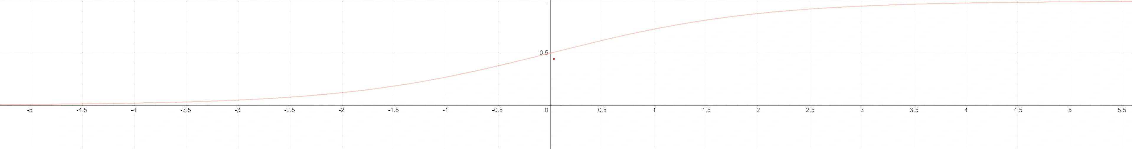
A standard sigmoid function
So that the new hypothesis function will output the probability toward one of the binary output(1/0) without overlapping.
Decision Boundary
We consider:
$$h(x) \geq 0.5 \rightarrow y = 1 \newline h(x) < 0.5 \rightarrow y = 0$$
Becuase of the bahavior of the logistic function:
$$\theta^{T}x=0, e^{0}=1 \Rightarrow h(x)=1/2 \newline \theta^{T}x \to \infty, e^{-\infty} \to 0 \Rightarrow h(x)=1 \newline \theta^{T}x \to -\infty, e^{\infty}\to \infty \Rightarrow h(x)=0$$
So that:
$$\theta^T x \geq 0 \Rightarrow h(x) = 1 \newline \theta^T x < 0 \Rightarrow h(x) = 0$$
Then you can just set $h(x)$ to 1 or 0 to get the decision boundary. For example:
$$\theta = \begin{bmatrix}5 \newline -1 \newline 0\end{bmatrix} \newline y = 1 ; \mathbf{if} ; 5 + (-1) x_1 + 0 x_2 \geq 0 \newline $Desicion Boundary: $x_1 \leq 5 $$
The plot should looks like:
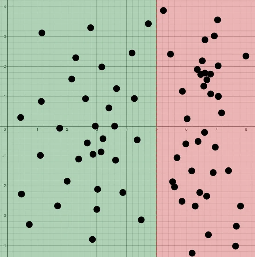
The green portion is “1” while the red($x_1>5$) is “0”